Why Retirement Planning Needs Monte Carlo Simulation

A retirement plan brings together several moving parts. There is the money already saved, the amount that may be added before retirement, the income expected later in life and the spending that needs to be supported.

That future income may come from several sources. A state pension might cover part of the household's essential expenses. A workplace or private pension may provide additional income. Some people may also receive rental income, an annuity or other regular payments. In some plans, these sources cover most or even all retirement spending. In others, savings and investments need to fill a large part of the gap.

Retirement planning usually starts by placing these elements on a timeline. We estimate future income, add the growth of current savings and future contributions, account for when different pensions become available and subtract the spending expected each year. The result is a projection showing how the person's finances may develop over time.

Investments are often modelled using an assumed average return. If the plan expects a portfolio to grow by 5% a year, the calculation applies that return year after year. The resulting line shows whether income and accumulated savings appear sufficient to meet future spending.

This is a useful starting point. It helps us check whether income, savings and spending fit together under a chosen set of assumptions. The problem is that the calculation usually applies the same investment return every year. Real investment returns arrive unevenly, and that unevenness can materially change a retirement plan.

John's plan provides a practical example.

• Age 45 today
• Plans to work until age 62
• £50,000 annual after-tax income
• £38,000 annual spending, split between needs and wants
• £250,000 saved across retirement and regular investment accounts
• State pension expected from age 68

The question he wants to answer is straightforward:

Can his current savings and future contributions support his spending throughout retirement?

Starting with an average return

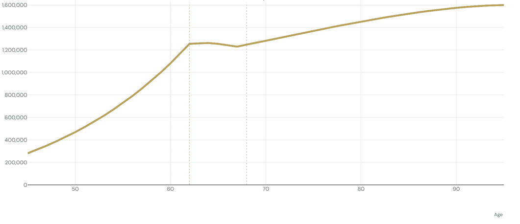
A traditional forecast might assume that John's investments grow by a fixed percentage every year. If the assumed annual return is 5%, the model applies 5% in the first year, another 5% in the second year and continues in the same way throughout his life.

This creates a smooth path. John's portfolio grows gradually while he is working and then changes direction when he retires and starts withdrawing money.

The calculation answers a precise question:

What would happen if John earned the assumed return every year?

That return may be a reasonable long-term estimate, but an average compresses many different years into one number. A market that rises by 18% one year and falls by 8% the next has an average annual return of 5%, but John never actually receives 5% in either year.

Percentages also build on one another. If £100 rises by 20%, it becomes £120. If it then falls by 10%, it becomes £108. The average of the two annual returns is 5%, but applying a steady 5% return for two years would produce £110.25.

The difference becomes more important when John is regularly adding or withdrawing money. While he is working, contributions are invested at different market prices. During retirement, spending must continue even after a poor investment year. Returns therefore interact with the timing of his cash flows.

An average return describes the journey as a whole. John's retirement depends on what happens along the way.

Why the order of returns matters

Consider two people who each start retirement with £100,000 and withdraw £10,000 at the end of every year.

Both experience the same two annual returns: one year of 20% growth and one year of a 10% loss.

The first person receives the positive return first. The £100,000 grows to £120,000, and after the first withdrawal £110,000 remains. A 10% loss in the second year reduces this to £99,000, followed by another withdrawal, leaving £89,000.

The second person experiences the loss first. The portfolio falls to £90,000, and the first withdrawal reduces it to £80,000. The following 20% gain brings it to £96,000, and the second withdrawal leaves £86,000.

Both people received exactly the same returns. The order alone created a £3,000 difference after only two years.

Over a retirement lasting thirty years, these differences can compound. Poor returns near the beginning of retirement can be particularly damaging because withdrawals continue while the portfolio is already falling. Later gains then apply to a smaller amount of money.

This effect is often called sequence-of-returns risk. The term simply describes the risk created by receiving investment returns in an unfavourable order.

John is especially exposed to this around retirement. His salary ends at 62, while his state pension starts at 68. During those six years, a larger part of his spending must come from his own savings. Strong or weak markets during this period can affect the rest of his plan.

A forecast based on one fixed return follows only one possible sequence. A Monte Carlo simulation allows us to examine many.

From one forecast to 10,000 possible paths

A Monte Carlo simulation repeats the same financial calculation thousands of times.

John's age, retirement date, income, spending, savings and pension remain the same. What changes from one calculation to the next is the path followed by investment markets.

In one scenario, John may experience strong returns during the years immediately before and after retirement. In another, retirement may begin during a prolonged market decline. Most scenarios will contain a mixture of positive, negative and average years.

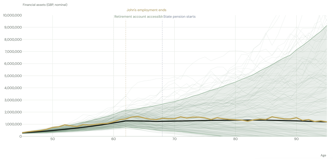
Each calculation produces one possible path for John's savings. Myriada repeats the process 10,000 times, creating 10,000 different versions of the same financial plan.

The purpose is not to select one of these paths as John's future. The collection of paths shows the range of outcomes that the plan can produce under the assumptions used.

This is similar to assessing the expected duration of a journey. Knowing the average travel time is useful, but a better plan also considers normal traffic, heavy traffic and unusually clear roads. The range helps us decide when to leave and how much extra time to allow.

For retirement, the range helps us understand how much room the plan has when investment conditions are less favourable than average.

What John's result means

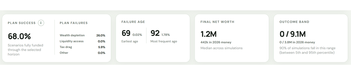
In John's simulation, 68% of the 10,000 scenarios fund all his planned spending through the end of the selected period.

In practical terms, around 6,800 simulated paths meet every planned cash requirement, while around 3,200 reach a point at which the available money can no longer cover the full amount.

The 68% result belongs to the assumptions used in the model. It depends on John's retirement age, spending, savings, contributions, pension income, taxes and the range of investment returns being simulated. Changing any of these inputs may change the result.

This makes the percentage useful for comparing decisions. John can see how the result changes if he works for one more year, saves more, reduces spending or changes the way his money is invested.

The percentage also needs to be read together with the timing of the unsuccessful scenarios.

John's earliest simulated shortfall occurs at age 69, but this happens in only 0.02% of scenarios. The most common age for the first shortfall is 92, when 1.78% of scenarios fail for the first time.

This tells John that the main pressure in his plan appears late in life. A small number of very difficult market paths create problems earlier, but most unsuccessful scenarios continue funding his spending for many years before falling short.

That distinction matters. A plan that can no longer support spending at age 69 presents a very different problem from one that first develops a shortfall at age 92. A single success percentage places both outcomes in the unsuccessful group, while the failure-by-age chart shows their practical severity.

Reading the range of outcomes

The wealth chart displays John's 10,000 simulated paths over time.

Every thin line represents one scenario. All paths begin at the same point because John's current savings are known. They gradually spread apart as each scenario experiences a different sequence of investment returns.

The dark central line shows the median outcome. The median is the middle scenario: half of the simulated outcomes finish above it and half finish below it.

The green area covers the range between the 5th and 95th percentiles. In simple terms, 90% of the simulated outcomes fall inside this area. Only 5% fall below it and 5% rise above it.

The band becomes wider as John gets older because small differences in early returns accumulate over time. A good year increases the amount available to benefit from later growth. A poor year reduces that base. After several decades, the difference between favourable and difficult paths can become very large.

In John's case, the middle outcome ends with around £1.2 million in future pounds. Myriada also shows this as approximately £442,000 in 2026 money.

The distinction accounts for inflation. A pound received several decades from now is likely to buy less than a pound today. "2026 money" translates future amounts into their approximate current purchasing power, making them easier to compare with John's present income and spending.

Across the middle 90% of John's simulations, final wealth ranges from zero to approximately £9.1 million in future pounds, or zero to around £3.8 million in 2026 purchasing power.

The width of this range is important. A forecast based only on average returns might show John one final balance. The simulation shows that the same plan can lead to wealth being depleted in difficult scenarios, while favourable scenarios can leave a substantial surplus.

From a forecast to a planning decision

The simulation gives John a more complete answer than a single projected balance.

His current plan funds all spending in 68% of the simulated scenarios. His savings are accessible before he stops working, and the model shows no failures caused by money being locked away when it is needed. The greatest pressure develops later in retirement, after many years of withdrawals, rather than immediately after he leaves work.

John can now test changes against the same 10,000-scenario framework.

He could retire at 63 instead of 62, giving himself another year of income and contributions and one fewer year of withdrawals. He could increase the amount saved while working. He could also use the distinction between his £30,000 of essential spending and £8,000 of discretionary spending.

For example, John may be comfortable reducing some discretionary spending after a particularly weak market period. A plan that allows spending to respond to circumstances may behave differently from one that assumes the full £38,000 must be withdrawn every year under every condition.

The useful question is therefore broader than whether 68% is a good or bad number. John needs to understand which changes improve the plan, what they cost him today and which risks they reduce.

Working for longer may improve the result, but it uses another year of his time. Lower spending may strengthen the plan, but it affects his lifestyle. A different investment mix may change both the potential gains and the possible losses.

Monte Carlo simulation makes these trade-offs visible because every version of the plan can be tested against the same broad range of market conditions.